Trading resolution for noise (on example of NEX-6)
Is dynamic range a number?
Measuring dynamic range of a camera may look like as a simple exersize: find the level of signal where
saturation is reached, divide by the level of signal where it becomes hidden by noise, and you are done.
However, while with contemporary designs of sensors, finding the saturation level is easy (at least
when you do not need an absolutely precise number), there are major problems when one
wants to find the second number.
The reason: while saturation cannot be undone by postprocessing, noise is changed in
postprocessing. Both intentionally, and as a side effect of downscaling the image. (If done correctly,
downscaling constructs an output pixel as a certain mix of input pixels, and mixing reduces the noise.)
So the question boils down to: exactly what is the workflow used before deciding that “the signal is hidden by noise”?
(There is another, unrelated, pitfall in the word “hidden”, but it is usually resolved by replacing this
with S/N ratio being 1. This definition, with contemporary sensors, makes the Poisson noise of photons/electrons
irrelevant: where S/N = 1, the Poisson noise is completely
swamped by the read noise of the sensor; so one may just consider the noise of a totally black source.)
For example, DxoMark decided that they measure noise after downsizing
to 8 Mpixels (with which algorithm?). This is fine if what you want is a print with this effective resolution
and you shy away from any noise reduction; however, a reasonable image processing workflow would include
some intelligent noise reduction. This noise reduction would be applied with selective strength: different
levels will be used for different (parts of) images. How much noise would remain depends not only on
the sensor, but also on the flavor and strength of the applied noise reduction.
To make the long story short: effectively, noise reduction trades resolution for noise; given a sensor,
one gets “noisiness” of the sensor not as a single number, but as a curve N(R): how much noise
remains when one is ready to give up the fraction R of resolution. Like this for NEX-6:
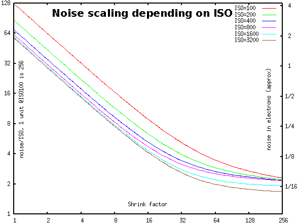
Here 1 electron is approximately 30 units on the left scale (and 1 step of ADC @ISO=100 is 256 units); higher ISO correspond to a lower curve.
Actually, the value at magnification=1 is extrapolated. The actual, pristine, noise on the color channel
is about 8% larger. This difference is due to the aggressive Lanczos filtering used in resizing.
Warning: The conversion of sensor’s units to electrons assumes full well of 33000e. Since I do not remember
where I took this number from, the scale on the right should be considered with a (tiny) grain of salt.
If one wants to get closer
to the real world, one would need to take into account the particular flavor of noise reduction. On
the other hand, to get an output pixel, any noise reduction algorithm, no matter how smart/adaptive/anisotropic it is,
would eventually select a certain region of the image, and would “average” input pixels in this region. So, to a certain
extent, the remaining noise is very similar to the noise averaged over a circle of the same area — which, in turn,
is very similar to the result of downscaling with an appropriate ratio.
And this is exactly what the graph above has as its horizontal axis: we just downscale with the provided
(linear) ratio, and measure the RMS noise of a color channel (of the totally black source). (These are RAW channels;
so Red and Blue count as 1 channel each, and Green as 2 channels.)
Boiling down: the “extinction” dynamic range
Thinking about this more: instead of investigating a whole curve, one also gets a very interesting number:
suppose that we are ready to give up ALL the resolution. How small is a signal which may be distinguished
from complete black? In this sort of game, we allow any algorithm of noise reduction, allow output images
of tiny sizes: how far can one go?! This number can be called the “extinction” dynamic range.
It is important to know this number for the “most general type” decisions on the digital workflow.
For example, an sRGB 16-bit image stores at most about 19.5EV dynamic range. So if the sensor is
able to produce an extinction dynamic range similar to this, one needs to use a better image format (or use tricks
like dithering — to write “between the levels of the output format” what one has read “between the levels of the ADC”).
The “extinction” dynamic range of NEX-6
I could go down to 19EV at ISO100: below in the center, the region exposed at saturation - 19EV is easily
distinguishable from darker regions:
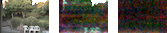
Left and center images are of the same scene, both downscaled 100x, but the center one had 13.5EV less exposure
(“corrected” in postprocessing: the brightness is increased 1`200`000%). With the exception of the sky, the brightest points on the left image are at saturation - 1.5EV.
Correspondingly, they are at saturation - 15EV on the center image (so the center image is underexposed
15 steps — with 12-bit sensor!). The right image is of a totally black scene; it is processed with the same workflow
as the center image (but with a different black point [0.26 lower] — this difference may be related to the fact that this image was taken 1 year later).
The rosemary bush (to the left of white chairs) is exposed at saturation - 5.5EV on the left image,
hence at saturation - 19EV on the center image. Compare it with much darker shadows on top of the
bush on the left image — and this distinction is preserved well on the center image.
A quick reminder: the exposure of 1 step of ADC of NEX-6 is 12EV below saturation.
So our -19EV is 1/128 of one step of ADC.
In the center and right images, we treated the row-averages separately (with a very
aggressive noise reduction), and treated the rest of the signal very mildly (the only noise reduction is a 50/50 mix with the
median-filtered image). Note: Even with such an aggressive noise reduction of row-averages, the discussed
features are almost hidden by horizontal noise-stripes (a purple one on top of white chairs, and an orange one on top
of the rosemary bush; there is also a white stripe near the top of the image); actually, one may need an extra 2x downscaling
to be absolutely sure that the difference between -19EV and “something yet darker” is real, and not
due to rich imagination.
The reason for our splitting away row-averages, and why it does not completely succeeds to remove the patterned
noise is explained below. It is related to levelling of resolution-vs-noise curves on the right of the graphs above:
it turns out that the reason for this levelling is the contribution of row-averaged noise; filtering this type of noise
more agressively helps in fighting this leveling.
Actually, the images are not scaled 100x down; instead every 2464×1638 channel is scaled 50% down, and 2 green channels
are mixed together. In particular, deBayering is not present in the workflow.
For completeness below are 5 images similar
to the right image above (taken within interval of several seconds). Since the main contribution is
1/f noise (which, unless
samples are overwhelming huge, is extremely unpredictable), the “pictures” of the noise are strikingly different.
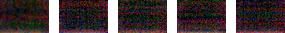
One can see here that the images are pure noise, so there was no light leak affecting our comparisons.
The lousy colors on both photos are due to a very simplified color processing pipeline:
we needed to work with output from raw converter which has levels equally-spaced; this precluded using any
smarts the raw converter knew how to do (multiplying integers with a fractional coefficient creates gaps in histograms, so
it should be better done after denoising — so we just skip matrix operations); the pipeline is described below).
Separating two sources of noise: row-noise and the rest
Looking at the graph above, a downscaling cannot reduce noise more than about 45 times, and this requires such a radical
downscaling that practically no details remain (to ≈25×16px). Above, we did show that on 50×33px images, one can achieve
a noise reduction of more than 64x. To understand how one can do it, we need to investigate the noise of the sensor in
much more detail (essentially, we investigate the most important features of the Fourier transform of the sensor noise — but
avoiding an explicit transform allows us to work with 1-dimensional data of the graphs above — instead of 2-dimensional
Fourier transform). Start with description of how the ADC actually works.
With the sensor of α700, Sony started a major shift in architecture of sensor’s ADC: for every column of image,
there is a comparator circuit. When scanning a row of image, one input of every comparator is connected to a
corresponding photocell, while the other input is connected to the output of a DAC (all in parallel). The DAC
generates a ramp staircase signal, and every comparator waits for the ramp to go over the output of the photocell,
and remembers on which step this would happen; this step becomes the output of ADC.
A similar architechture is used on NEX sensors.
This architecture allows the integration times for comparators to be extremely long (relative to other architecture), of
order of tens of microseconds, which allows a significant reduction of noise. Adding this to independent comparators at every
column, correlated part of the noise of comparators practically disappears (0.03 electron or less). As a result, the
noise is to a very significant extent a white (=patternless) noise (so good for an eye); this is reflected in the graphs
above decreasing linearly (with slope 1) for a long time.
However, eventually, when one averages over larger and larger regions, the curves start to flatten out. Visually,
this correspons to the noise acquiring a certain pattern. For other (“pipelined”) sensors architectures, the patterns consists of
stripes going in the direction of scanning the photocells (due to 1/f noise). For per-column architectures, the noise is a mix
of noises from two sources: NDAC and NC: the noise of DAC, and the noise of the comparator.
As explained, NC is for all practical purposes a white noise; on the other hand, NDAC is shared
by all the photocells in a row, so leads to horizontally-striped noise. (Compare with the downscaled pure-noise images
above — they are dominated by NDAC even after significant noise reduction!).
It is trivial to split any image into row-averaged part, and the rest. One can immediately see that two sources of
noise would affect these parts separately (for all practical purposes). In particular, one can measure these two contributions to the
read noise separately (shown with the same conventions as above):
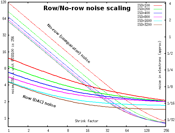
The slower descending (bold) curves are NDAC, the steeper (thin) curves are NC. (Combining two independent
sources of noise, in the first approximation the magnituude of the total is the maximum of two. This effect is very
easy to see comparing two diagrams above: of the total noise, and of two components.)
In case of purely white noise the NC curve would have slope -1, and NDAC — slope -0.5
(since they are for 2-dimensional and 1-dimensional distributions). The lower four NDAC curves have a certain
part on the left behaving like this. However, the top two NDAC curves have a noticable curvature everywhere.
This is due to higher proportion of 1/f noise for NDAC with ISO100 and ISO200. The strength of this noise is
reflected on the slope of the graph near the right edge.
This picture explains why with the photo above, one needs much more aggressive noise reduction of NDAC
noise than of NC noise: -19EV at ISO100 corresponds to 1/128 of 1 step of ADC, or
2 vertical units on the graphs above. One needs to reduce noise about 64 times, so do at least 64x shrinking (actually,
more than this, since the graphs are levelling out at such shrink factors!). And
at this place of the graphs, NDAC noise is much stronger than NC noise. To get below 2 units (total) with
shrinking factor 50 (of a color channel; so the overall shrinking is 100x w.r.t. de-Bayered image), one needs only small
extra reduction of NC (corresponding to an extra 2x downsizing), but the needed reduction of NDAC is
stronger than what is possible with
any resizing. Hence the baroque chain of medians and resizings documented below.
For all ISO numbers except 400 and 800, when shrinking up to 32x the banded structure of noise should not be noticable
(NDAC < NC). However, for ISO400 and ISO800, the banding becomes pronounced a little bit earlier than this.
Smoothing out fluctuations in the measured noise
How did we get the curves shown above? On one hand, they are just approximations to the image statistics
extracted from images made with a camera. On the other hand, a lot of collected data is dominated by so-called
1/f noise; this is an extremely “nasty” kind of noise with a very
strong component on very low temporal frequencies. There is a certain low-frequency cut-off; and unless you collect
data on periods significantly larger than this characteristic time, your measurements of noise are going to vary a lot. The
inspection of data represented below shows that the cut-off is between shrink=256 and
shrink=512. Since every image contains only about 1500 rows, the variation between images is still significant.
On the other hand, 5 images taken together contain about 7500 rows; so one expects that a sample of 5 images gives reasonable
approximation to the actual noise.
Moreover, below we fit curves simultaneously for 6 values of ISO. Effectively, this increases the pool of data,
and increases statistical significance of our analysis.
In short: these curve form a reliable representation of “a less reliable” stats collected from 30 images (5 per ISO).
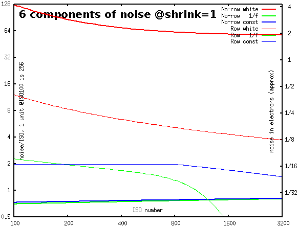
Fine structure of every curve
It turns out that every curve can give a really good approximation by combining 3 independent
sources of noise: white noise (would descend linearly on the graphs above), 1/f noise
(with power descending linearly with log(shrink_factor), and a smooth pattern noise (which
does not decrease with shrinking). So to describe every curve, one needs to specify
3 numbers: strength of white noise at magnification=1, how much the 1/f noise decreases with
every 2x step of magnification, and the strength of the smooth pattern noise (it is given
by the value of 1/f noise on the right edge of the graphs). On the graph
below they are for NDAC noise, as fitted by gnuplot:
As we said before, the values at magnification=1 are slightly larger than the
fitted curve. (These values were not used during fitting.)
5 images were analysed for every value of ISO.
The common wisdom is that the ISO1600 and ISO3200 looks suspiciously like they
are obtained by digital amplification of ISO800. These diagrams show that as far as
NDAC is concerned, these behave very differently from ISO800 (and
have a significantly lower noise). Comparing with the first diagram (one for combined noise), one can see
that this difference is significant for the combined noise too.
These graphs have two very strange features: first, note convergence of graphs for ISO100…ISO800
on the right, and sudden improvement in smooth pattern noise when going to ISO1600 and ISO3200. Second, the power of 1/f noise
decreases to 0 (linearly in log(downscale)), then remains 0 for ISO1600 and ISO3200. We know no possible explanation for this…
Now do the same for NC; however, since it changes on much larger scale, we draw the graph
with different values on the vertical axis: instead of “just” noise, we plot noise*shrink_factor.
This replaces straight lines with slope -1 by horizontal lines (on the left), and replaces levelling with
bending up (on the right), and makes it possible to see the details on the right much better:
For NC, there is practically no difference between ISO 800 and ISO1600, ISO3200;
compare the tiny difference for the white noise component (on the left) with practically no difference in 1/f and smooth pattern
components (on the right).
While the white noise component (and maybe 1/f component) depends on ISO (at least between 100 and 800), it looks like
the smooth pattern component does not depend on ISO at all.
Appendix: workflow
The workflow for the (majorly) underexposed photos was:
dcraw -4 -v -k 120 -b 256 -S 4215 -W -T -h -M -o 0 -r 1 1 1 1 DSC00014.ARW
set resize=-statistic median 1x3 -statistic median 1x3 -resize 71% -statistic median 1x3 -statistic median 1x3 -resize 71%
set resizeX=%resize% -statistic median 1x3 -statistic median 1x3
set resize50=-resize   16% ( +clone -resize 1x! ) ( +clone -resize 394x! ) ( -clone 0,2 xc:gray50 -poly "1,1 -1,1 1,1" -resize 12.5% ) -delete 0,2 ( -clone 0 %resize% %resize% %resizeX% ) -delete 0 xc:gray50 -poly "1,1 1,1 -1,1"
convert DSC00014.tiff -size 2464x1638 xc:#606850 -maximum xc:#a098a0 -minimum %resize50% -evaluate subtract 30028 -channel B -evaluate subtract 262 -channel G -evaluate subtract 48 +channel -set option:compose:args 70,30 -compose blend ( +clone -evaluate subtract 62 ) -composite ( +clone -evaluate subtract 155 ) -composite -channel R -evaluate multiply 2.945313 -channel B -evaluate multiply 1.312500 +channel -evaluate multiply 144 -evaluate pow 0.4545 DSC00014.tiff-2perc-blackpoint3e.png
convert ! ( +clone -statistic median 3x3 ) -set option:compose:args 50,50 -compose blend -composite median3-!
The workflow to get the stats (of totally-black photos) after downscaling (with 3 different output directories for: “as is”; row averages; residual after removal of row averages):
set odir=.....
for %f in (*.ARW) do ( dcraw -4 -v -b 16 -T -h -M -o 0 -r 1 1 1 1 -k 0 -S 4095 -c %f | convert - -verbose -channel R -separate -write info:%odir%%f-id             -write info:%odir%%f-id0 -resize 50%% -write info:%odir%%f-id1 -resize 50%% -write info:%odir%%f-id2 -resize 50%% -write info:%odir%%f-id3 -resize 50%% -write info:%odir%%f-id4 -resize 50%% -write info:%odir%%f-id5 -resize 50%% -write info:%odir%%f-id6 -resize 50%% -write info:%odir%%f-id7 -resize 50%% info:%odir%%f-id8 )
for %f in (*.ARW) do ( dcraw -4 -v -b 16 -T -h -M -o 0 -r 1 1 1 1 -k 0 -S 4095 -c %f | convert - -verbose -channel R -separate -write info:%odir%%f-id -resize 1x! -write info:%odir%%f-id0 -resize 50%% -write info:%odir%%f-id1 -resize 50%% -write info:%odir%%f-id2 -resize 50%% -write info:%odir%%f-id3 -resize 50%% -write info:%odir%%f-id4 -resize 50%% -write info:%odir%%f-id5 -resize 50%% -write info:%odir%%f-id6 -resize 50%% -write info:%odir%%f-id7 -resize 50%% info:%odir%%f-id8 )
for %f in (*.ARW) do ( dcraw -4 -v -b 16 -T -h -M -o 0 -r 1 1 1 1 -k 0 -S 4095 -c %f | convert - -verbose -channel R -separate -write info:%odir%%f-id ^( +clone -resize x1! -resize x2464! ^) xc:gray50 -poly "1,1 -1,1 1,1" -write info:%odir%%f-id0 -resize 50%% -write info:%odir%%f-id1 -resize 50%% -write info:%odir%%f-id2 -resize 50%% -write info:%odir%%f-id3 -resize 50%% -write info:%odir%%f-id4 -resize 50%% -write info:%odir%%f-id5 -resize 50%% -write info:%odir%%f-id6 -resize 50%% -write info:%odir%%f-id7 -resize 50%% info:%odir%%f-id8 )
Massaging stats into a table suitable for gnuplot:
egrep "deviation" *-id* >stats2
perl -w010l00pe "s{\n^\w+.ARW-id\d+:[\s\w]+:\s+([\d.]+).*}{\t$1}mg; s{\s\([\d.\x25]+\)}{}g" stats2 >stats2-l
perl -wlne "@f=split /\t/; $iso = int(($.-1)/5); print qq($iso\t$_\t$f[$_+1]) for 0..$#f-1; print q(); print q() unless $.%5" ! > !-tbltbl
My command processor replaces ! by the name of the currently selected file.
gnuplot commands:
aaa00           = 69.7672
bbb00           = 56.222
pz              = 1.21546
noise_norow_white(x,y)=(aaa00/2**(pz*y)+bbb00)/x
bbbb            = 0.0891347
bbbL            = 0.00538994
noise_norow_1_f(x,y)=sqrt(-(bbbb+bbbL*y)*(log(x) - 8*log(2)))
vvv88           = 0.53485
vvvv88          = 0.022412
ww88q           = 0.00157777
noise_norow_const(y)=sqrt(vvv88 + y*vvvv88 + y*2*ww88q)
nnr(x,y)=sqrt(noise_norow_white(x,y)**2+noise_norow_1_f(x,y)**2+noise_norow_const(y)**2)
aa00            = 726.538
bb00            = 2.23045
noise_row_white(x,yy)=sqrt(aa00/x)/((yy)+bb00)
bbb             = 28.9846
ys              = 5.66972
bp              = 1.97286
yp              = 0.000332662
ypp             = 16
noise_row_1_f(x,y)=sqrt(-bbb/(ys+y+yp*ypp**y)**bp*(log(x) - 8*log(2)))
vv88            = 1.97449
ll88            = 2.99808
dd88            = 0.273942
noise_row_const(y)=(vv88 - (y < ll88 ? 0 : (y)-(ll88))*dd88)
nr_(x,y,yy)=sqrt(noise_row_white(x,yy)**2+noise_row_1_f(x,y)**2+noise_row_const(y)**2)
nr(x,y) = nr_(x,y,y>4?4:y)
set logscale xyy2 2
set title "Row/No-row noise scaling" offset 0,-3 font "bold,20"
set xlabel "Shrink factor" offset 0,3.5
set ylabel "noise/ISO, 1 unit @ISO100 is 256" offset 10,0
set y2label "noise in electrons (approx)" offset -15,0
set y2tics border nomirror add ("1/2" 0.5, "1/4" 0.25, "1/8" 0.125, "1/16" 0.0625, "1/32" 0.03125)
set ytics border nomirror
set y2range [.7/30:128./30]
set label "No-row (comparator) noise" at first 4,50 rotate by -42 font "bold,12"
set label "Row (DAC) noise" at first 1.7,2.5 rotate by -17 font "bold,12"
plot [1:256] [y=0.7:128] nnr(x,0) lt 1 title "ISO=100 ", nnr(x,1) lt 2 title "ISO=200 ", nnr(x,2) lt 3 title "ISO=400 ", nnr(x,3) lt 4 title "ISO=800 ", nnr(x,4) lt 5 title "ISO=1600", nnr(x,5) lt 6 title "ISO=3200", nr(x,0) lt 1 lw 2 title "", nr(x,1) lt 2 lw 2 title "", nr(x,2) lt 3 lw 2 title "", nr(x,3) lt 4 lw 2 title "", nr(x,4) lt 5 lw 2 title "", nr(x,5) lt 6 lw 2 title ""

noise(shrink,iso)= ( y=log(iso/100)/log(2), sqrt(nnr(shrink,y)**2+nr(shrink,y)**2) )
set y2range [1./30:128./30]
set title "Noise scaling depending on ISO" offset -2,-3 font "bold,20"
unset label
plot [shrink=1:256] [y=1:128] noise(shrink,100) lt 1 title "ISO=100 ", noise(shrink,200) lt 2 title "ISO=200 ", noise(shrink,400) lt 3 title "ISO=400 ", noise(shrink,800) lt 4 title "ISO=800 ", noise(shrink,1600) lt 5 title "ISO=1600", noise(shrink,3200) lt 6 title "ISO=3200"

set y2range [.5/30:128./30]
set title "6 components of noise @shrink=1" offset -10,-3 font "bold,20"
set xtics 100, 2
set xlabel "ISO number" offset 0,3.5
plot [y=100:3200] [0.5:128] noise_norow_white(1,log(y/100.)/log(2)) lt 1 lw 2 title "No-row white", noise_norow_1_f(1,log(y/100.)/log(2)) lt 2 lw 2 title "No-row   1/f", noise_norow_const(log(y/100.)/log(2)) lt 3 lw 2 title "No-row const", noise_row_white(1,log(y/100.)/log(2)) lt 1 title "Row white", noise_row_1_f(1,log(y/100.)/log(2)) lt 2 title "Row   1/f", noise_row_const(log(y/100.)/log(2)) lt 3 title "Row const"
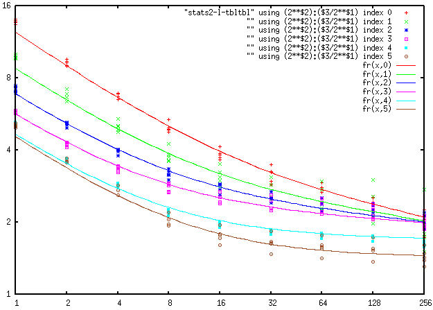
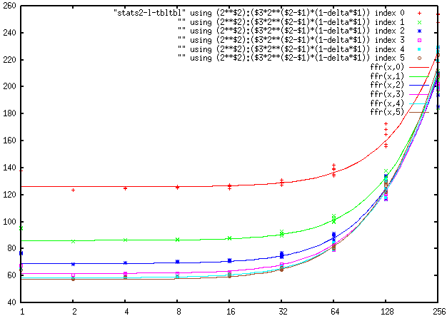
gnuplot commands including actually measured noise:
plot "stats2-l-tbltbl" using (2**$2):($3/2**$1) index 0, "" using (2**$2):($3/2**$1) index 1, "" using (2**$2):($3/2**$1) index 2, "" using (2**$2):($3/2**$1) index 3, "" using (2**$2):($3/2**$1) index 4, "" using (2**$2):($3/2**$1) index 5, fr(x,0) lt 1, fr(x,1) lt 2, fr(x,2) lt 3, fr(x,3) lt 4, fr(x,4) lt 5, fr(x,5) lt 6
gnuplot was not able to automatically fit to the values above; I needed to start with
ys=6; bp=2; ypp=16; yp=0 and refit several times, creatively combining with
fit [64:256] log(nr(x,y)) "stats2-l-tbltbl" using (2**$2):-2:(log($3)-column(-2)*log(2)):(1) via vv88,ll88,dd88
fit  [2:256] log(nr(x,y)) "stats2-l-tbltbl" using (2**$2):-2:(log($3)-column(-2)*log(2)):(1) via aa00,bb00,bbb,vv88,ll88,dd88,ys,bp,yp,ypp
The particular forms of functions used to “fit” dependence of every component of noise
(white, 1/f, const)
on ISO number is not important. After one knows a good fit, much simpler functions could be used. (For example,
for (the largest — for low shrink factors) “No-row White” component, the dependence on ISO can be described well as
C'+C/ISO.) Below are the graphs of what every one of 6 components (as fitted by gnuplot) contributes
at shrink factor 1 (depending on ISO):
As above, what is plotted is the interpolated values at shrink=1; the actual, unfiltered, noise of a color channel is 8% higher.
For the 1/f noise, we plot the increment “in power” when “doubling resolution” (so between shrinking
factors 2N and N).
Hence contribution of 1/f noise at shrink factor 1 is 2√2 times larger than the plotted value (since there
are 8=log₂ 256 doubling steps between 1 and 256, and 8x increase “in power” means 2√2 = √8 increase in magnitude).
For const noise, we assume that 1/f noise cuts-off at the shrink factor 256. (Trivia: recall that
1/f noise has infinite power at low frequencies; so in reality, it is always cut off below a certain frequency.
If one underestimates this frequency, this corresponds to increasing the const noise; overestimating
may lead to “negative” const noise — which is easy to recognize.)
For no-row flavor, and low-ISO of row-flavor, note how close are the plots of the 1/f noise and
the const noise. This suggests that if one cuts-off 1/f noise at the shrink factor 512,
the const noise would disappear (so shrink=512 is the “real” cut-off as opposed to “artificial”
cut-off at shrink=256).
And for higher ISO of the row-flavor, the “real” cut-off gradually decreases to about shrink=256.
Comparing to white noise, the 1/f + const noise gives smaller contribution into the row noise
for ISO up to 400 (at shrink=1). For larger ISOs, they are of similar magnitude. At ISO=100,
the 1/f noise becomes the largest contributor in the row noise only for
shrink≥4.
Suppose we do not care about separation of noise into row/non-row flavors (so all we need is to analyse
dependence of total noise on the shrink factor). Since two flavors
of const noise, and two flavors of 1/f noise have the same dependence on the shrink factor, one can
combine components in every pair. Then only 4 components remain: no-row white, decreasing as 1/shrink, row-white, decreasing
as 1/√shrink, 1/f, decreasing as √log₂(256/shrink), and const. One gets a formula
√(C₁/shrink² + C₂/shrink + C₃log₂(256/shrink) + C₄).
Appendix II: mysteries of the total noise
It is needless to say that to function well, a good denoiser must know which parts of the scene are pure noise,
and which are not. So it must know the complete model of noise of the camera. One should either provide the denoiser
with massive tables of data, or design a model describing the noise of the camera using just a few numbers.
The standard model of the read noise of the sensor is to imagine the data flow as: sensor → amplifier → ADC,
with both “arrows” contributing a certain amount of noise (n₁ and n₂). Changing ISO changes the amplification (call it N), so the total
noise is a combination of Nn₁ and n₂, with N proportional to ISO number. Plotting the dependence of noise on ISO, one can
separate the contributions of the pre-amplifier noise n₁ and the post-amplifier noise n₂.
(Trivia: some cameras have a two-stage amplifier, which reflects on graphs of noise vs ISO. Then the analysis is
applicable to the “better” ISO numbers, when the noise of the “bad” stage is minimal.)
Very small ISO numbers and very high ISO numbers are usually “faked” by an extra step of (post-ADC) digital amplification.
Such amplification does not change the ratio noise/ISO, so is visible as straight-line-through-0 pieces of the graph
which do not match the curve “in between”. This is why we omit ISO≥1600 below (after looking on the graphs including
these data!).
If the pre-amplifier and the post-amplifier noise are uncorrelated, the total noise is √(C₁ISO²+C₂); this is
what fits the graphs of many cameras. However, if these noises are fully correlated (e.g., caused by noise on the power line),
then the total noise is C₁ISO+C₂. Let’s see how it looks for NEX-6 (measured data and best fits by models):
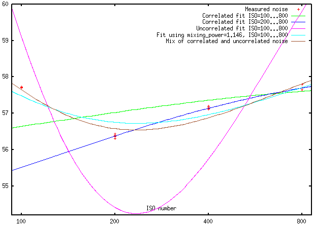
To make the scattering of measured values visible, we use a vertical unit dependent on ISO number. So
the vertical axis is in “certain abstract units”. Note also that this axis has a very narrow range; the difference between
top and bottom is only 10%.
One can see that the “uncorrelated noise” model does not fit the data at all. Moreover, between ISO 200…800, the “correlated
noise” model gives a practically ideal fit. And the quality of that fit cannot be matched by “any reasonable model” if one wants
to extend the range to ISO=100!
What may be an explanation of this? I suspect that the BLUE “correlated noise” model is the matching model, and the difference
of 4% in the predicted value of noise at ISO=100 may be explained by something like “the ISO=100 is actually ISO=108” or some such.
(Some people measure “actual ISO” of the camera versus the “advertaized ISO”; I did not find these data for NEX-6, so cannot
check this conjecture.)
Appendix III: possible usage
Currently, I’m instrumenting dcraw with a possiblity to use the investigated models of noise in its
“wavelet denoising” option. While going down to -19EV with this algorithm is out of question, the data above
suggests that the algorithm should be able to trade noise vs. resolution down to -17EV wihout a major overhaul.
To do better, one should be able to take into account the separation of row and no-row noise. And here one hits a
major hurdle present in real high-dynamic-range photos, but avoided in the severely underexposed photos we used above:
to separate the row-noise, one needs the “dark” regions to take a significant portion of a row they touch. Depending on
composition, this may be so: one may have a bright sky above, and a dark bottom half of the image; then one should be
able to separate row noise in the bottom half of the image. But for many compositions, such a separation won’t be possible,
and the last EV (or two) near -19EV won’t be reachable.
In short: the denoiser should be able to special-case the “horizontally stretched” dark areas, and separate the
row noise for such areas. Other dark areas, where separation is not possible, will have smaller “extinction” dynamic range.
Above, our workflow allowed us to ignore the camera’s optical system mapping the subject to an image on the sensor.
It is not clear whether it is able to create an image with such a dynamic range, 19EV. Since
most people think that it is not possible to extract such a dynamic range from the sensor, it may happen that this
question is not yet investigated.
Ilya Zakharevich nospam-abuse@ilyaz.org